Shortcut on the Way to Freeform Optics

Download

Shortcut on the Way to Freeform Optics

Published in: Kunststoffe International 12/2013, page 58-61

Authors: Lars Dick (Jenoptik Polymer Systems GmbH) und Laura Florez

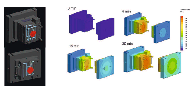
Virtual Mold Trials. The manufacture of plastic optical components usually involves a highly iterative process during development of the molded part and mold construction. Reason for this is the uncertainty associated with the injection molding behavior. The case example from a research project demonstrates how a virtual mold trial can replace this stepwise approach, which also results in considerable cost reductions.


Optical components manufacturing is one of the most demanding tasks for injection molding. Precise dimensions, tight tolerances, and the persistent demand for faultless and reproducible parts represent the operational framework in this industry. Driven by increasing miniaturization and more functionality in new device generations in the past years, the industry has shown a strongly increasing demand for high-precision injection molded optical components. Analogous to the innovative impulses for new, more compact equipment system triggered in recent years through the functional options of aspheres, new perspectives for future system innovations are presently emerging through the use of application-specific freeform optics. This nomenclature summarizes refracting and reflecting surfaces that clearly differ from symmetric and aspheric geometries.

However, due to inadequate availability of technical basics, today's demand for plastic types for freeform optics can only be met at uneconomic expense. Within the scope of the FREE project – the acronym stands for “precision  freeform optics” – Jenoptik Polymer Systems GmbH in Triptis, Germany, was faced with the challenge of producing symmetric, non-rotation freeform optics from high-performance plastic materials. Hereby, the aim was to achieve a precision of 0.5 µm. In order to penetrate this lucrative business, in which polymerbased precision optics with  symmetric, non-rotation freeform profiles play a key role, this project was to create the required basic competences.

Matching the Process for Freeform Surfaces
For optic components made of plastic, manufacturers have a basic choice between replicative methods of injection or compression molding, and material removal methods of ultra-precision diamond machining. While ultra-precision machining methods are typically used for small to medium-sized batches – i.e. characteristic for prototyping tasks –, replicative molding methods are only employed in series production because of the high
preparatory costs. These costs mainly include the complex production of the master molds, which requires a considerable advance investment, and, due to the only vague knowledge of the injection molding process, frequently involve several iterative loops.

For non-symmetric freeform surface profiles the machined implementation of the complex geometry in a ductile mold material with the necessary optical quality as well as the necessary measurement technology are very complex.The investigation and determination of process conditions during injection molding for these precise requirements is a so far unsolved task.

In this case, the simulation tool “Sigmasoft Virtual Molding” (Sigma Engineering GmbH in Aachen, Germany) was
used to analyze the influence of different process parameters on component quality. For every step in the calculations, the molded parts and the replication mold are closely coupled. Calculations for form filling are based on the complete 3-D Navier Stokes flow equations. These are followed by a true 3-D calculation of post-pressure and cooling phase, plus component shrinkage and deformation until room temperature is reached.

After an initial thermodynamic consideration, a mold heat-up time is determined, followed by a count of the cycles
required until thermal equilibrium is reached, which is essential for an expedient replication process. Various key aspects are examined in the following simulations of the filling process:

  • Flow fields,
  • pressure and temperature distribution in the melt at different points in time,
  • development of the flow front during mold filling,
  • possible locations of weld lines and air pockets,
  • representation of mold filling and flow phenomena behind the flow front by means of (massless) tracer particles.

Following the simulated filling phase, the
cooling and post-pressure phase is examined, whereby temperature distribution during the cooling phase is in the
forefront, in order to determine an optimum residual cooling time. Subsequently, shrinkage and deformation in
all spatial directions are determined and
displayed.

Thermal Analysis of the Mold
At first, a thermal simulation is used to establish for how long hot water at 90 °C must flow through the mold's tempering channels until the target temperature or a thermodynamic equilibrium is practically reached (Fig. 1). Initially, the mold absorbs a great amount of energy. After about 10 minutes,the energy input is considerably lower, but a stationary condition has not yet been reached. After a 30-minute heat-up time with 90°C hot water, a homogeneous temperature distribution between 86.5 and 86.8 °C is noticeable in the cavity. Therefore, this
time should be allowed in the practical tests (Table) before the first molded part is produced.

On the other hand, the manufactured parts generate a cyclic thermal input to the overall thermodynamic system, in accordance with the established balance equation:
Qmelt + Qtempering = Qcomponent + Qradiation

Accordingly, the amount of energy introduced by the melt (Fig. 2) and the mold's tempering channels equals the sum of energy removed by the molded part and through heat radiation of the mold. If the sum of all these energy flows does no longer changes, the system exhibits the same energetic state before and after the cycle. Consequently, it has reached a quasi-stationary state, and production of good parts can commence. For example,
if it takes 30 cycles to reach this state of equilibrium, the first 30 parts of every test series must be seen as scrap. Useful measurements can only be made from the 31st part onward.

Analysis of Filling Behavior
The filling simulation is followed by a thermal investigation of the replication process. Hereby, possible jetting, flow
lines as well as air pockets can be detected. The homogeneous filling process determined by the simulation correlates closely with the results of the injection tests (Fig. 3). For the practical comparison, a filling study was conducted, whereby only a defined portion of material is injected into the mold, which is not enough for complete mold filling. For the first part in the diagram, 17 cm3 of shot volume remain in the dosing unit, and only 3.5 cm3 for the last part.

The simulation shows how melt temperature changes during the filling phase. Here, one sees clearly that some surface areas of the component near the gate cool down significantly,whereby temperatures of 130 °C are reached. Because of the long filling time, a temperature difference results in the component at the end of the filling phase (Title figure). An explanation for this can also be provided by the simulation, where the flow conditions behind
the flow front are shown by so-called tracer particles (massless particles). It shows clearly that in several areas near the gate the melt flow is slower and cools down more quickly than in areas in which the plastic is still subjected to high shearing forces or hot melt continues to enter the mold.

Post-pressure and Freezing Behavior
Noticeable in the simulated pressure distribution of the component is that the adjusted post-pressure of 1,000 bar only exists on the nozzle side of the gate. With increasing distance from the gate, the effective pressure drops. At the beginning of the post-pressure phase, 968 bar are measured in the component at a distance from the gate, and 975 bar near the gate. At the end of the post-pressure time, pressure distant from the gate is only 600 bar, and 622 bar near the gate (Fig. 4). In a next step, component freezing can be simulated (Fig. 5). This is highly relevant, as this simulation provides reliable findings regarding post-pressure time and residual cooling time. A constant post-pressure only has a positive effect on molding accuracy as long as a liquid core can be maintained between gate and component.

Frozen areas are shown transparent. Red areas are still molten and are are affected by post-pressure. Blue areas are still molten, but can no longer be supplied with post-pressure. Here, only the attained pressure is relevant for compensating the plastic’s volume shrinkage. The component can be affected by dwell pressure up to some 90 % of frozen volume. After 30 s of post-pressure time, the necessary connection to the lens is frozen, so that a longer post-pressure time for increased molding accuracy makes no sense (Fig. 4, right). Therefore, the originally defined post-pressure time was increased from 20 to 30 s in the course of the investigations.

In the post-pressure phase, only very low shear values and also lower temperatures occur. This leads to a strong increase in viscosity during the post-pressure phase. In turn, high viscosity means that it becomes more difficult to press melt into the mold. What does the simulation reveal about cooling time? For this, temperature across the component cross-section was initially analyzed 100 s after the filling process (value calculated with a Fourier
transform). As shown in Figure 6, the central region is almost at 118 °C, and therefore still above the glass transition temperature. After the defined residual cooling time of 180 s, and a dwell time of 30 s (cooling time = 210 s), the temperature in the central region has dropped to about 94 °C, and therefore below the Vicat softening temperature (103 °C), while the border regions of the freeform surface are at 89 °C, i.e. almost at cavity temperature. 30 minutes after demolding, the component’s core temperature has reached 25.3 °C, i.e. practically room temperature.

Finally, deformation is examined. Across the diameter (44 mm) the surface shrinks almost uniformly by 180 µm. This
equals a shrinkage of 0.41 %,which is very close to the measured shrinkage of 0.3 %. Also in the comparison of mean deformation as a function of dwell pressure, the measured and predicted values correlate very well (Fig. 7).

Summary
Today, the manufacture of optical components often involves complex iteration loops before the production starts. Sigmasoft Virtual Molding can predict the interactions between process parameters and component quality. This permits development time and costs to be saved. Moreover, the cause for undesirable defects can be detected and eliminated at an early stage.